


What makes someone great at their job is rarely what they knew before starting. It's usually what they learned through their experience on the job itself. A new analyst learns which numbers the partners actually check, and a new associate learns what each client likes about the contract they drafted. None of that is written down anywhere. It comes from their experience. Enterprise agents face the same problem: every company has its own definition of good work and all of it keeps shifting as new kinds of requests arrive. The goal of continual learning is to let models scale on this experience axis, just as people do, specializing to the work in front of them. And just like when you're tasked with something on the job, you can only rollout once!
But modern RL recipes aren’t built to use traces from productionized agents for RL. Group-based algorithms often require trajectories generated from identical environments, on the exact same task. Trained-critic algorithms require expensive multiples on inference costs, and are hard to train, and aren’t robust to changes in the grader itself.
The other hurdle is that trajectories and their rewards arrive to a training batch with no labels on what type of task the agent handled, and “type” of task might even be more complex than some discrete classes of tasks. FlashREINFORCE (FlashRF) [Hu et al., 2026] is a recently proposed algorithm which baselines tasks with the batch mean of reward, and performs well even in asynchronous settings, requiring neither batches nor a trained critic.
So how do you learn from a task you can only run once? In this post, we look at ways to train on a single rollout per task, then present our method, GS1, which achieves state-of-the-art results on knowledge-work benchmarks without repeated rollouts.
Baseline Estimate
To eliminate the need for groups, we first need to understand why they exist in the first place. We start with a fundamental concept underlying many modern reinforcement learning algorithms: the baseline estimate.
Setup: A task is one prompt together with its environment. The policy is the model (actor) being trained, parameterized by weights . A rollout is an attempt at a task (the messages, tool calls, and final results). A grader scores the rollout with a reward , normalized between 0 and 1 in our setup. A training step uses a batch of rollouts indexed by , so rollout attempts task and earns reward . A baseline is an estimate of the typical reward a rollout from earns (more on this soon!). The advantage is the reward centered by the baseline.
Most policy-gradient methods weight each rollout by its advantage rather than its reward [Williams, 1992; Sutton et al., 2000]:
The baseline is a core part of policy optimization because it helps the model learn which attempts were better or worse than expected. Rollouts that beat the baseline (the policy's usual reward on that task) become more likely in the next iteration of the policy, while those that fall short become less likely.
Importantly, any baseline that doesn't depend on the rollout being scored leaves the expected policy gradient unchanged:
This means a good baseline can reduce the variance of the gradient, making training more stable without introducing bias.
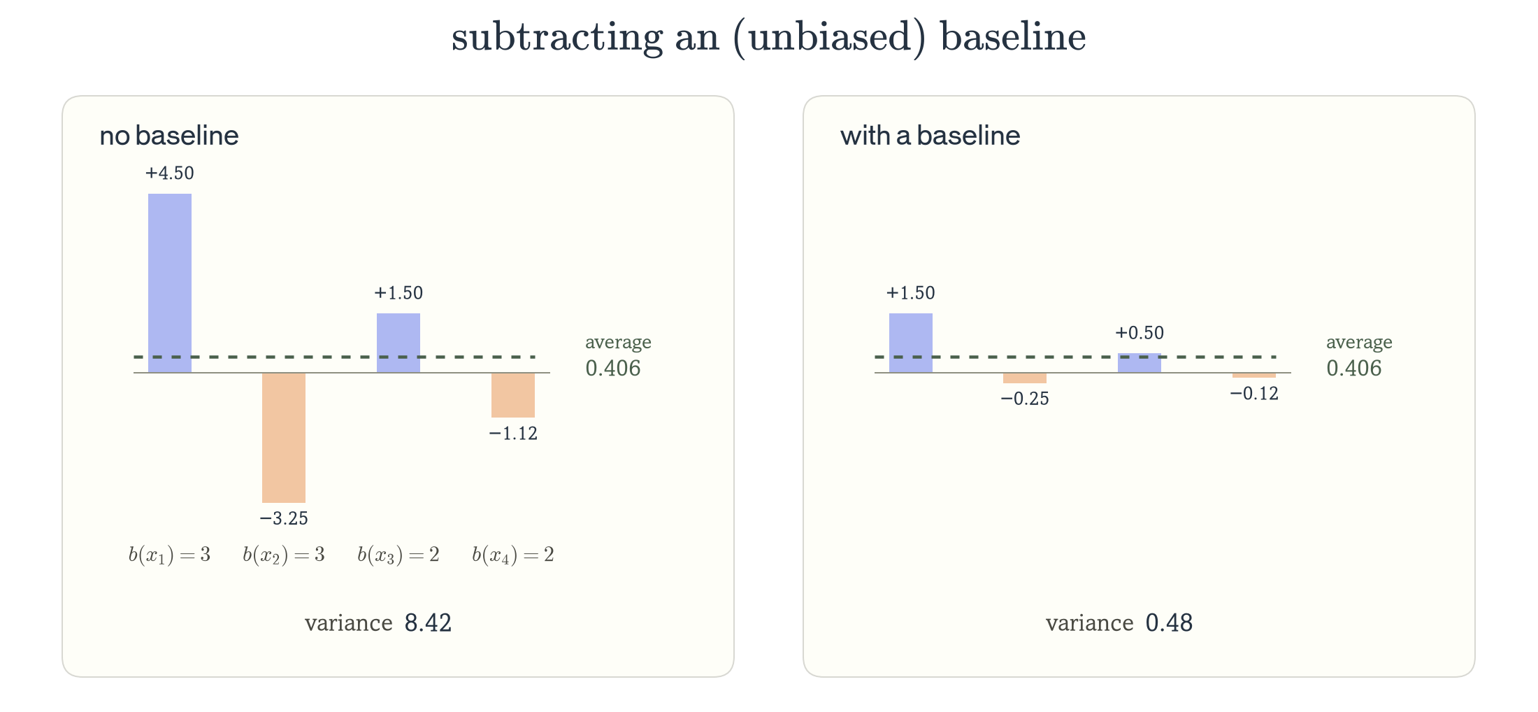
This brings us to the central question: how do we obtain the baseline?
Ideal baseline estimate
A natural choice is the model's expected reward on a task, averaged over all possible rollouts under its current policy [Greensmith et al., 2004]:
An agent might take millions of possible paths through a task, each producing a different reward. We cannot evaluate every possible rollout to determine the true expected reward.
Instead, we need to estimate the baseline from limited experience (rollouts).
Group-based baselines
GRPO [Shao et al., 2024] takes a straightforward approach to baselining: run the same task multiple times.
For each task , GRPO samples rollouts, collectively called a group. Each rollout receives a reward , and its advantage is calculated by subtracting the group's average reward and normalizing by its standard deviation:
The intuition is simple: if a model performs better than the other rollouts in its group, we reinforce that behavior. If it performs worse, we discourage it. As the group size grows, its average reward then becomes a more accurate estimate of the model's expected reward on that task.
But groups come with a fundamental constraint: we need to be able to run the same task multiple times under identical conditions.
This is straightforward in controlled environments, where it’s possible to reset the state and replay a task. But this becomes much harder in production, where an agent interacts with live users, changing APIs, and external systems that cannot be reset.
Critic-based baselines
PPO [Schulman et al., 2017] takes a different approach to estimate the baseline. We attempt to approximate the baseline by training a model directly to estimate the expected final reward at a point in the rollout.
The critic's prediction becomes our baseline, allowing us to calculate the advantage directly:
Here, is the true return observed from state , and is the critic's predicted expected return [Schulman et al., 2016]. The benefit of this is that we can estimate advantages from a single rollout, without needing to repeat the same task.
But this introduces a different problem: the critic itself needs to be trained.
For long agentic trajectories, learning an accurate critic is difficult. A reward may only arrive after the agent has taken hundreds of actions, which make intermediate states quite hard to evaluate. Then, errors in the critic can introduce noise and bias into advantage estimates, making training less stable [Yuan et al., 2025].
There is also a computational cost. In LLM training, the critic is often comparable in size to the policy itself, adding substantial inference costs.
The goal: Group-free and critic-free
We've seen two approaches to estimating a baseline. GRPO compares multiple rollouts of the same task, meanwhile PPO trains a critic to predict expected rewards. Both have limitations when learning from real-world experience.
Our goal is to find a third approach: can we derive a useful baseline estimate from a single rollout, without needing groups or a trained critic?
| Method | Group-free | Critic-free |
|---|---|---|
| GRPO | ✗ | ✓ |
| PPO | ✓ | ✗ |
| Our goal | ✓ | ✓ |
FlashREINFORCE: Batch-based estimate
What if, instead of comparing multiple rollouts of the same task, we compared rollouts from different tasks?
This is the idea behind FlashREINFORCE [Hu et al., 2026], which builds on the batch-level reward normalization introduced by REINFORCE++ [Hu, 2025].
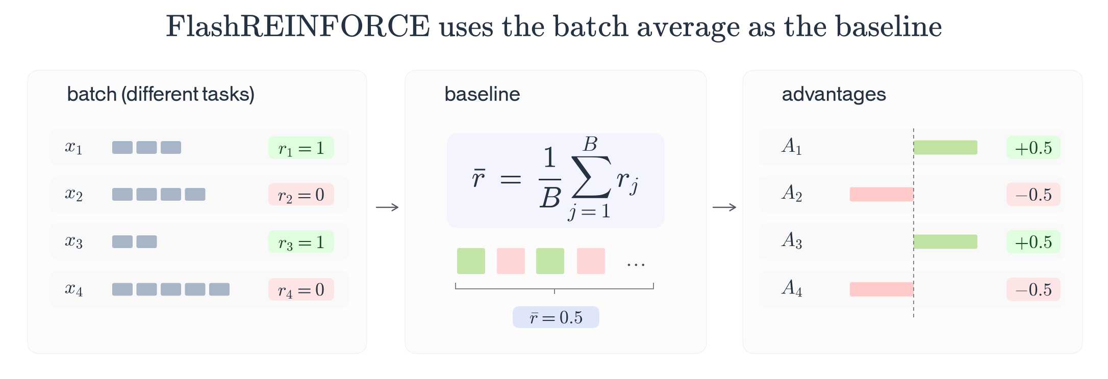
Recall that GRPO estimates a baseline by averaging the rewards of multiple rollouts from the same task. FlashREINFORCE instead uses the average reward across an entire training batch, where each rollout can come from a different task.
For a batch of rollouts, the advantage becomes:
Here, is the reward for rollout , and is the number of rollouts in the batch.
This gives us a baseline without repeating tasks or training a critic. FlashREINFORCE combines this with a token-level training objective and a KL penalty to stabilize policy updates [Schulman, 2020]. No groups or critics involved!
We now have an approach that is both group-free and critic-free. But is the batch average a good baseline for every task?
Where the batch-based estimate breaks
FlashREINFORCE uses the same baseline for every task in a batch, but also tasks can vary substantially in difficulty.
Consider a finance agent that is correct 90% of the time for extracting revenue from a 10-Q, but is correct only 10% of the time at building a five-year financial model. If the batch average reward is 0.5, then both tasks receive the same baseline, despite having very different expected rewards. We suspect that production traces have a similar structure too, where there are frequently requests where the agent almost always completes, right next to other requests the agent almost never completes.
The batch average captures how well the model performs across tasks, but it doesn’t describe how well it is expected to perform on a particular task.
To understand how much task difficulty varies in practice, we sampled multiple rollouts per task using Inkling-Small across several public benchmarks.
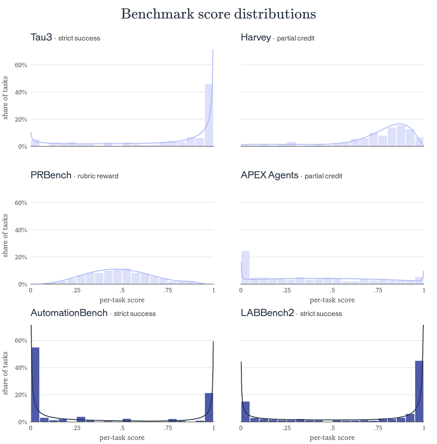
We observe substantial differences in task-level expected rewards across benchmarks. Some distributions do have a single dominant mode, while AutomationBench and LABBench2 show a pretty large separation between tasks the model always solves and tasks it never solves.
This suggests that a single batch-wide baseline could miss important differences in task difficulty.
GS1: Constructing soft groups
Formalizing intuition about good baselines
We've seen that task difficulty can vary quite a bit, and that a single batch average might not be a good baseline for every task. In order to improve upon FlashREINFORCE’s concept of a batch, we must be able to assess the quality of a baseline.
To do so, we propose a new metric, effective batch size. The idea is to measure how much variance a baseline adds to the policy gradient, and express that in terms of how many rollouts we would need with a perfect baseline to get the same variance.
Let's start with the ideal baseline. For any task , let be the average reward the current policy would get if it attempted that task many times. We don't know this value in practice, so we estimate it with a baseline .
The difference between a rollout's reward and its baseline can be split into two parts:
Computing the variance of the advantage:
With rollouts the gradient's variance, under certain assumptions (Appendix A), becomes:
where is the typical squared size of . A perfect baseline () with rollouts would reach variance . Finally, setting the two equal gives us:
This is the effective batch size.
For example, if we're training with 32 rollouts and our baseline is perfect, the effective batch size is 32. If the baseline adds as much variance as the natural variation within tasks, the effective batch size falls to 16. We'd need twice as many rollouts with that baseline to reach the same approximate gradient variance as a perfectly baselined batch of 16.
Measuring effective batch size in practice
We can estimate effective batch size offline, without running RL. For our experiments, we use the starting policy and a batch size of .
- Collect calibration rollouts. Sample 8 responses per task from the starting model, so we can estimate how much its rewards vary on each task.
- Measure within-task variance. Compute by averaging the reward variance across tasks. This tells us how much variation remains even with a perfect baseline.
- Simulate training batches. Randomly sample 32 different tasks and take one rollout from each. For every rollout, compute its baseline using only the other 31 rollouts, just as we would during training.
- Measure baseline error. Compare each predicted baseline with the task's average reward, estimated from its other 7 calibration rollouts. We subtract to account for noise in that estimate, giving us .
- Calculate effective batch size. Plug both measurements into .
We now have a way to measure how good a baseline is without running RL. With this, we can start looking at how to improve on the batch average, using what we know about the difficulty of different tasks.
Task-specific baselines
FlashREINFORCE showed that we can learn from a single rollout per task without training a critic. But its batch-wide baseline treats every task as equally difficult.
What if we could estimate each task's baseline using other tasks of similar difficulty, without needing multiple rollouts of the same task?
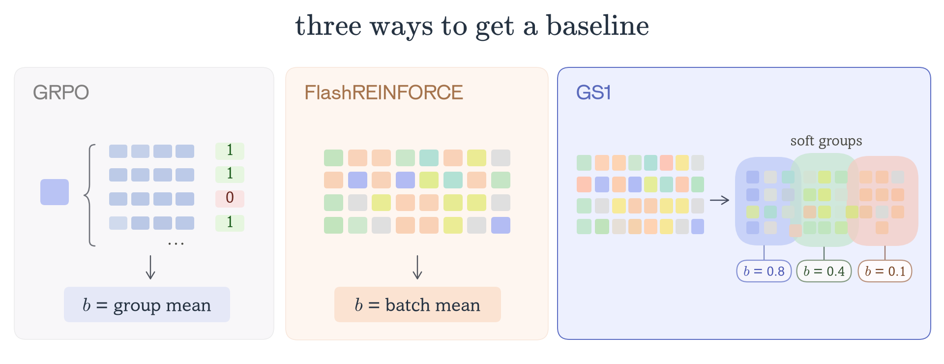
We propose GS1 (Group Size 1), a group-free, critic-free algorithm that estimates task-specific baselines by constructing fuzzy groups of similar tasks within a training batch.
Each task receives its own baseline, without requiring additional rollouts or a trained critic.
Estimating a baseline from similar tasks
GS1 builds on FlashREINFORCE's training objective, changing only how the baseline is estimated.
Instead of averaging rewards equally across the batch, we estimate a baseline for each task using a similarity-weighted average of other rollouts:
Here, is the reward of another rollout, and determines how much that rollout contributes to task 's baseline.
Tasks that are expected to have similar rewards receive higher weights, while less comparable tasks receive lower weights. This creates the concept of soft groups, where each task draws from a different, potentially overlapping set of comparisons, rather than belonging to a fixed cluster.
We then calculate the advantage as usual:
From our effective batch size formulation, we know that a better baseline is one that gets closer to each task's expected reward. The goal is therefore to find a way of weighting other tasks that reduces this error, and in turn increases effective batch size.
This brings us to the important question of how we determine which tasks are similar.
What makes two tasks similar?
We're not necessarily looking for tasks with similar content. Crucially, we're looking for tasks on which the current policy is expected to achieve similar rewards.
Let denote the expected reward of the current policy on task . We want to estimate from features available before the rollout is sampled.
The best prediction of using only these features, in the mean-squared-error sense, is:
This metric gives us a way to characterize what makes a useful set of features. Then by the law of total variance:
The first term describes how much variation in expected reward the selected features can explain. And the second measures what still remains unpredictable in those features.
A useful kernel is one where features explain a large part of the variation in expected reward across tasks.
We can evaluate the effectiveness of kernels offline using the metric of their estimated effective batch size, as described in Appendix B.
Results
Our goal is to train an agent that learns from the work it already does, where we can only see one rollout from each task once. We test the various algorithms on four benchmarks that represent knowledge work: legal analysis (Harvey LAB [Grupen et al., 2026]), professional legal and financial reasoning (PRBench [Akyürek et al., 2025]), business workflow automation (AutomationBench [Shepard and Salimans, 2026]), and scientific research (LABBench2 [Laurent et al., 2026]). In every run, each training rollout comes from a different task, just like it would in production.
We explore two questions: First, can a group-free baseline learn just as well as GRPO, which replays each task several times? Second, when tasks have wide variance in difficulty, does GS1's task-specific baseline improve on FlashREINFORCE's shared batch mean baseline?
All runs were trained with Inkling-Small (276B total parameters, 12B active) with the same number of rollouts per step. GRPO samples 8 rollouts per task, so a 32-rollout step covers 4 tasks, while FlashREINFORCE and GS1 cover 32. The results report performance on held-out tasks, and Appendix E describes each benchmark in further detail.
Learning without groups
The first question we explore is whether groups are necessary at all. If one rollout per task is enough to learn from, then an agent can train on production traffic without replaying anything.
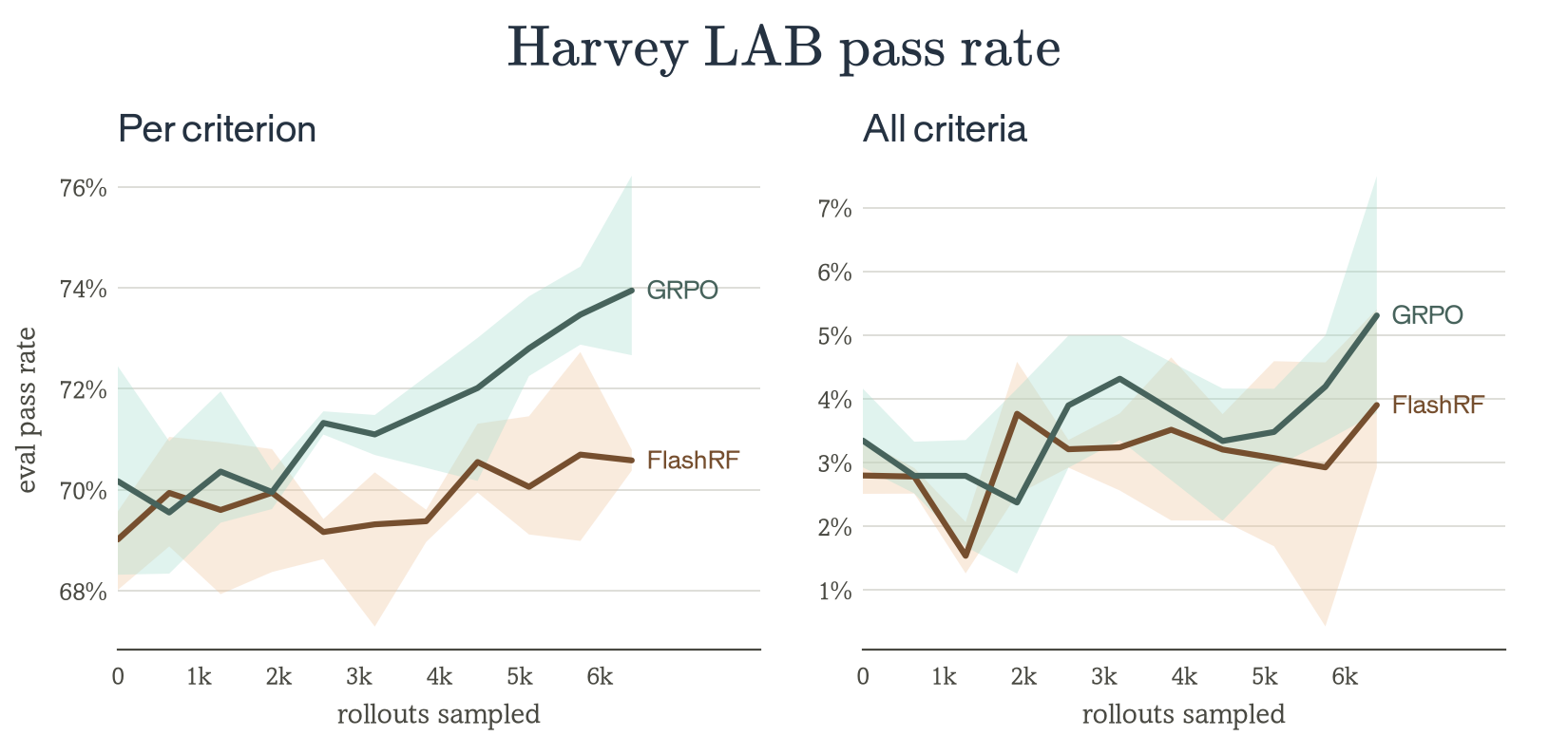
On Harvey LAB, we find that FlashREINFORCE improves held-out pass rate just as well as GRPO does, with one rollout per task and no critic. Legal work is a domain where tasks can't be replayed in production, so this is the setting where a group-free method has to hold up.
On PRBench, FlashREINFORCE actually does better than GRPO, improving held-out rubric score by 2.0 points against 0.8. Most of the difference comes from out-of-domain tax and cross-border structuring tasks. In this case, covering 32 tasks per step instead of 4 appears to matter more here than a precise baseline (Appendix D).
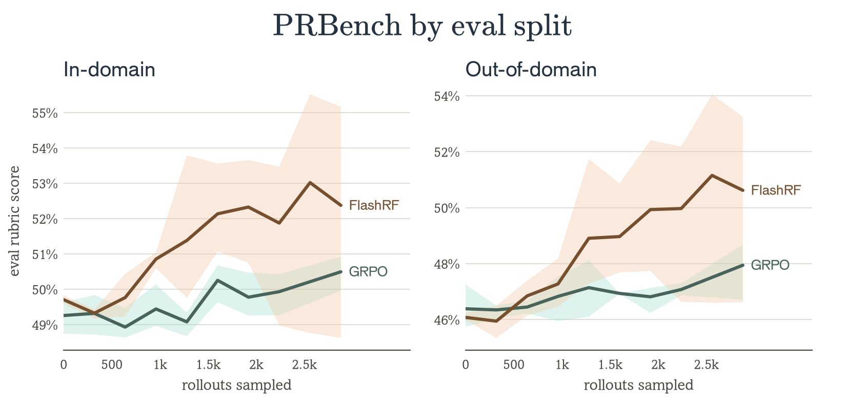
Together, these results show that training on knowledge work does not require replaying tasks, and it’s possible to get comparable results by only rolling out once. That already removes the main obstacle to training on production traffic. But, one critical limitation is that the batch mean gives every task the same baseline, and we saw earlier that difficulty can vary widely within a benchmark.
GS1 on heterogeneous tasks
In practice, production traffic is rarely uniform. An agent is oftentimes completing tasks that it can do extremely easily, and then right afterwards handling a request that it struggles with every time, and that mix is where a shared baseline is most wrong.
LABBench2 and AutomationBench both have this structure. On each benchmark, many tasks are ones the starting policy almost always solves or almost always fails, so the batch mean sits far from most tasks' expected reward. This is where GS1's task-specific baseline helps provide stability to the training run.
On LABBench2, GS1 improves held-out pass rate from 63% to 68%, and remains stable throughout training. FlashREINFORCE climbs alongside it early, but then slips to 65% late on in training while GS1 stays at 68%.
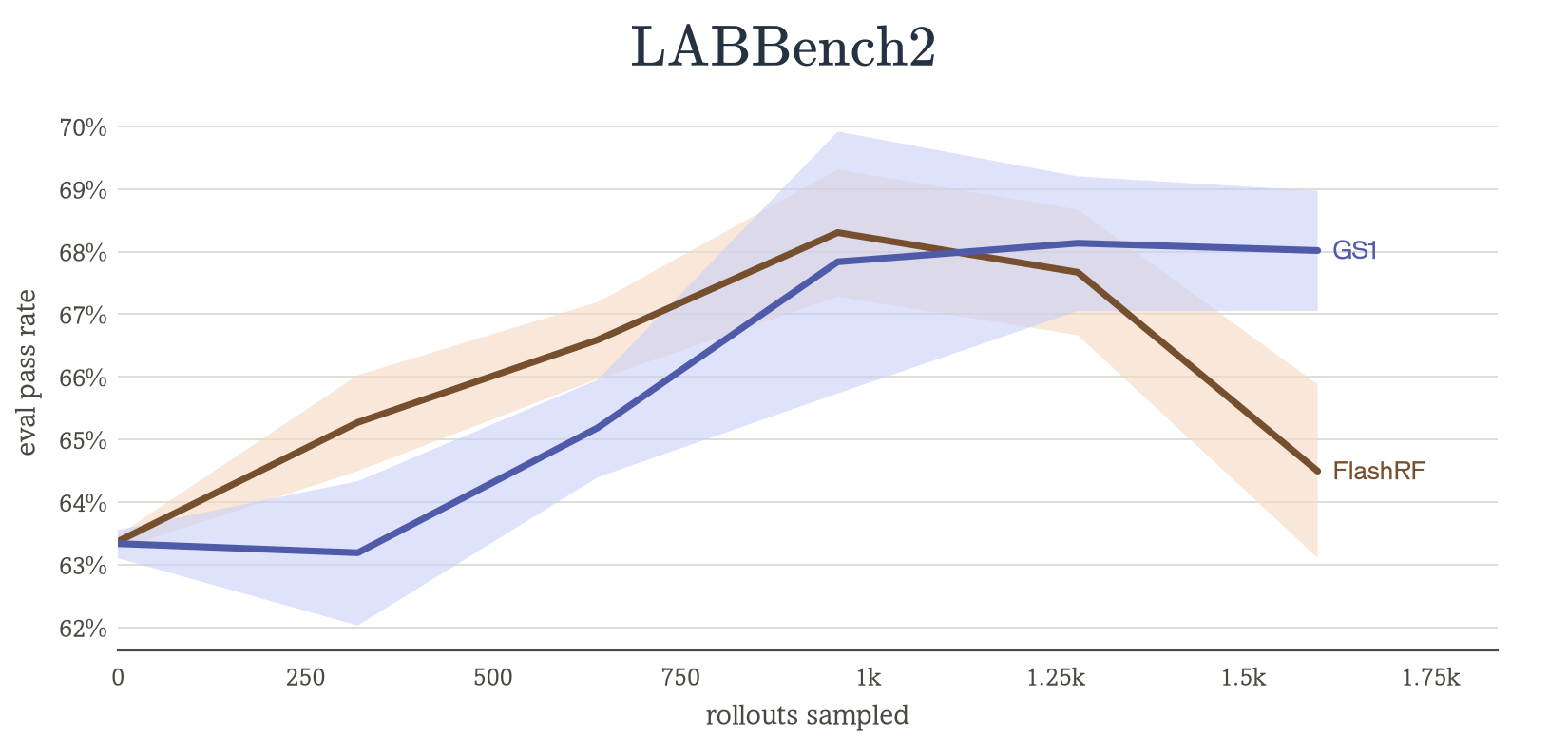
A continual learner has to keep what it learns as training goes on. Over a long run, GS1 keeps its gains where the shared baseline starts to give them back.
AutomationBench tests a second kind of robustness, to the learning rate. At a tuned learning rate of and 32 rollouts per step, all three methods reach similar final performance.
| GS1 | FlashRF | GRPO |
|---|---|---|
| 21.0% | 19.5% | 21.4% |
| Eval pass rate | Eval pass rate | Eval pass rate |
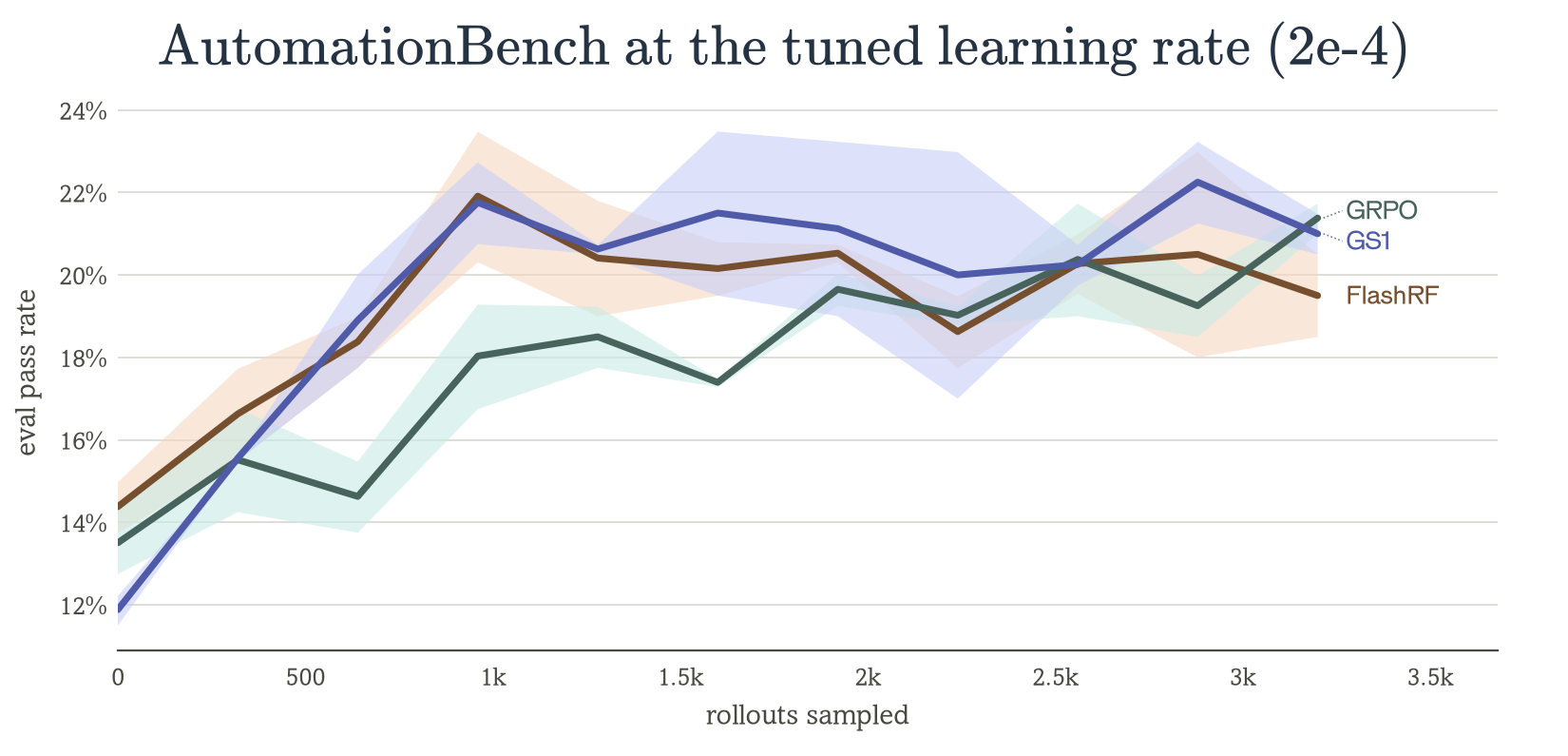
GS1 matches GRPO without replaying a single task. GRPO's 32-rollout step covers 4 distinct tasks, while GS1 spends all 32 rollouts on different tasks.
The methods separate when we raise the learning rate.
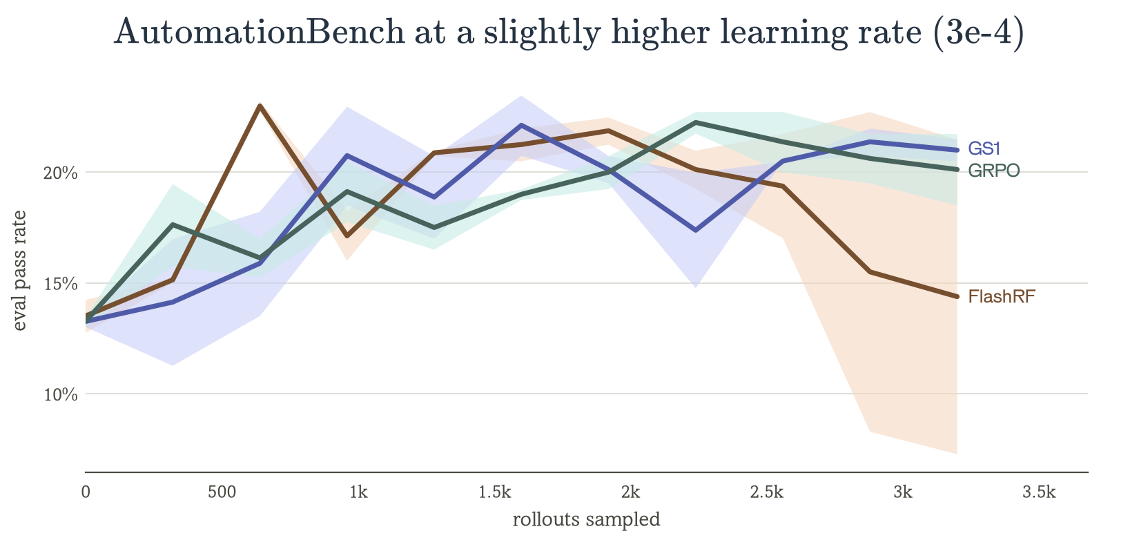
FlashREINFORCE's pass rate falls from 21.7% to 7.2% after roughly 2,500 rollouts, while GS1 and GRPO stay stable. Estimating a baseline that is wrong for most tasks produces noisy gradients, and a larger step size amplifies that noise.
Across both of these benchmarks, GS1 is the more robust method. A continual learning system can't retune its learning rate every time the mix of incoming work shifts, and so it needs a method that remains stable across long runs and across settings.
Baseline quality stabilizes training
Clearly, the GS1 baseline performs far better at higher learning rates (and we hypothesize, smaller batch sizes), when the high variance FlashRF advantages destabilize training.
At a batch size of 32:
| Benchmark | FlashRF | GS1 | Improvement |
|---|---|---|---|
| AutomationBench | 9.3 | 13.0 | 1.39× |
| LABBench2 | 10.9 | 12.6 | 1.16× |
| Harvey LAB | 23.8 | 24.4 | 1.02× |
| PRBench | 5.2 | 5.3 | 1.03× |
On AutomationBench, FlashREINFORCE's batch of 32 is effectively worth only 9.3 perfectly baselined rollouts. GS1 raises that to 13.0, a 39% improvement without collecting any additional rollouts. This is also where GS1 shows the clearest improvement in training stability.
But why does GS1 help so much on AutomationBench, while barely improving on LABBench2, Harvey LAB, or PRBench?
When similarity helps, and when it doesn't
We've seen that GS1 works by using similar tasks to estimate a baseline. But this is only useful if the similarity tells us something about how difficult a task is for the model.
Consider a simple example where tasks are from two groups: easy and hard. Let represent which group a task belongs to, with average rewards and .
If we knew which group each task belonged to, we could simply give easy tasks one baseline and hard tasks another baseline, and that would be much better than using the same batch average for both.
In practice, we don't know the group difficulty or baseline directly. We only have the task features , such as the prompt, to attempt to predict it.
The best estimate of a task's expected reward from these features is formulated as:
This is just a weighted average of the easy and hard rewards, based on how likely the task is to be an easy one.
We can then measure how much the features contribute to distinguishing the two groups:
There are two things that matter here. First, how different the rewards are between easy and hard tasks. Second, how much the features help us tell those tasks apart.
We can describe the second part using mutual information:
This measures how much knowing the features reduces our uncertainty about whether a task is easy or hard.
At one extreme, if , then these features tell us nothing about the task’s difficulty. In this case, every task gets the same predicted probability , and the baseline trends back toward the batch average.
At the other extreme, if , then the features perfectly distinguish easy from hard tasks. And we can recover the full between-group variance, , that a shared baseline would miss.
This explains why GS1 helps more on some benchmarks than others, depending on the success of the kernel.
On AutomationBench, easier tasks seem to share recognizable prompt characteristics, meaning the kernel can use these to distinguish them from harder tasks and estimate better baselines.
LABBench2 also has a large difference between easy and hard tasks, but they look much more alike to our similarity features. The kernel has a harder time telling them apart.
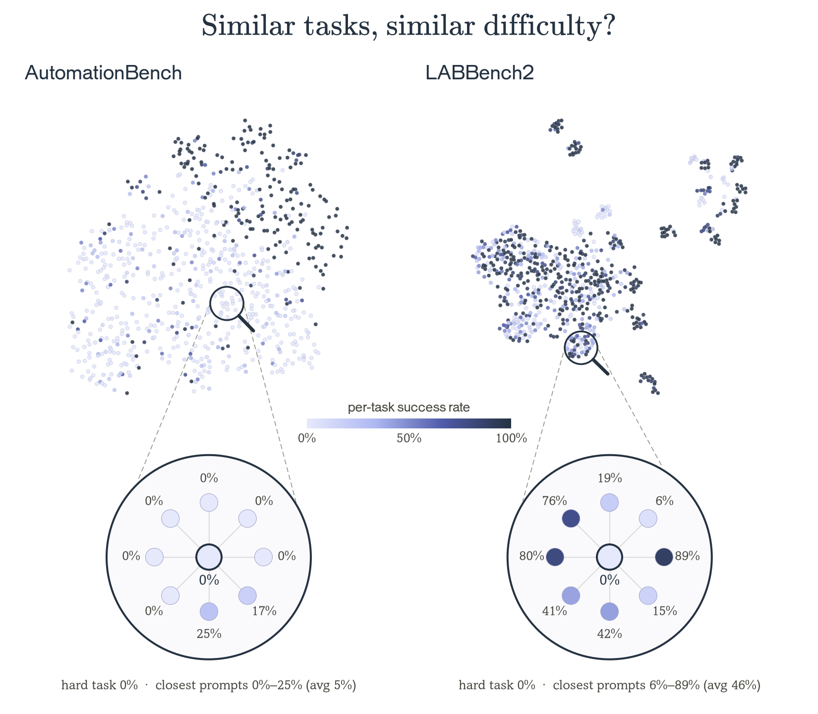
We see this in the effective batch size measurements. GS1 improves effective batch size by 39% over the batch mean on AutomationBench, and by 16% on LABBench2.
That GS1 still trains more stably on LABBench2 suggests even a modest improvement in the baseline matters over a long run. AutomationBench shows how much more is available when the features line up with difficulty.
This also suggests where to improve GS1. Right now, our kernel only sees the initial task information. In production, we often have more context, like the customer, workflow, or documents involved. If those features help predict how difficult a task is, we can use them to build better baselines.
Where this goes
The goal of this work is to train on experience from the real world that can't be replayed. We show that across four knowledge-work benchmarks, a baseline built from the batch can learn from one rollout per task, with no groups and no critic. Where task difficulty varies and can be described by a kernel, GS1's task-specific baseline estimate remains stable over long runs and holds even when the learning rate changes.
From here, there are several future directions to explore:
- Kernels that can explain more of the task variance. The entire space of GS1 kernels is largely underexplored. Currently, our kernels see only the agent’s starting configuration and prompt. LABBench2’s results find that this isn’t always enough, so perhaps there are other signals we can derive.
- Credit assignment within a trajectory. GS1 gives us one baseline per trajectory, so every turn of a long run shares the same advantage. Instead, we could develop per-turn baselines that stay group-free and critic-free so that we have more fine-grained steering of the model.
- Difficulty as a signal. GS1's baseline is an estimate of how well the current policy does on each task. The same estimate could be used to decide which traces experts should review, or show a team where its agent is weakest.
Trajectory
GS1 removes the need to replay a task, and the metagraders from our companion post on Continual Grading remove the need for a verifier. By combining these two insights, a team can train on the traces its agent already has produced, without needing to first build an environment that copies its customers' systems. Both are available as a research preview on Trajectory.
We're hiring researchers and engineers to work on continual learning from real-world experience. If that's the problem you want to work on, join us.
Citation
Please cite this work as:
Vemuri, Nikhil; Yap, Dian Ang; Trajectory Labs. “You Only Rollout Once.” Trajectory Labs: Field Notes, November 2026. https://trajectory.ai/field-notes/you-only-rollout-onceOr use the BibTeX citation:
@misc{trajectory2026yoro,
  author       = {Vemuri, Nikhil and Yap, Dian Ang and Trajectory Labs},
  title        = {You Only Rollout Once},
  howpublished = {Trajectory Labs: Field Notes},
  month        = {November},
  year         = {2026},
  url          = {https://trajectory.ai/field-notes/you-only-rollout-once},
}
References
- Akyürek, A. F., Gosai, A., Zhang, C. B. C., et al. (2025). PRBench: Large-Scale Expert Rubrics for Evaluating High-Stakes Professional Reasoning. arXiv:2511.11562.
- Greensmith, E., Bartlett, P. L., and Baxter, J. (2004). Variance Reduction Techniques for Gradient Estimates in Reinforcement Learning. JMLR 5, 1471–1530. Paper.
- Grupen, N., Pereyra, G., and Pereyra, J. (2026). Open-Sourcing Harvey's Long Horizon Legal Agent Benchmark. Harvey. Blog post.
- Hu, J. (2025). REINFORCE++: An Efficient RLHF Algorithm with Robustness to Both Prompt and Reward Models. arXiv:2501.03262.
- Hu, J., Zhang, Y., et al. (2026). FlashREINFORCE: Critic-Free Single-Rollout Asynchronous RL for Agentic Language Models. NVIDIA. PDF.
- Laurent, J. M., Bou, A., Pieler, M., et al. (2026). LABBench2: An Improved Benchmark for AI Systems Performing Biology Research. arXiv:2604.09554.
- Schulman, J. (2020). Approximating KL Divergence. Blog post.
- Schulman, J., Moritz, P., Levine, S., Jordan, M., and Abbeel, P. (2016). High-Dimensional Continuous Control Using Generalized Advantage Estimation. ICLR. arXiv:1506.02438.
- Schulman, J., Wolski, F., Dhariwal, P., Radford, A., and Klimov, O. (2017). Proximal Policy Optimization Algorithms. arXiv:1707.06347.
- Shao, Z., Wang, P., Zhu, Q., et al. (2024). DeepSeekMath: Pushing the Limits of Mathematical Reasoning in Open Language Models. arXiv:2402.03300.
- Shepard, D., and Salimans, R. (2026). AutomationBench. arXiv:2604.18934.
- Sutton, R. S., McAllester, D., Singh, S., and Mansour, Y. (2000). Policy Gradient Methods for Reinforcement Learning with Function Approximation. NeurIPS. Paper.
- Williams, R. J. (1992). Simple Statistical Gradient-Following Algorithms for Connectionist Reinforcement Learning. Machine Learning 8, 229–256. Paper.
- Yuan, Y., Yue, Y., Zhu, R., Fan, T., and Yan, L. (2025). What's Behind PPO's Collapse in Long-CoT? Value Optimization Holds the Secret. arXiv:2503.01491.
- Zhou, H., Ye, K., Xu, E., Zhu, J., Yang, Y., Gong, S., and Shi, C. (2026). Demystifying Group Relative Policy Optimization: Its Policy Gradient is a U-Statistic. arXiv:2603.01162.
Appendix
A. Deriving effective batch size
In the single-rollout setting, a batch has distinct tasks , rollout earns reward , and is how well the policy does on task on average. The update is
where is rollout 's response. Subtracting doesn't change what we're estimating, as long as is chosen without looking at :
Assumption 1 (the baseline never sees the rollout it scores). This holds by construction for every baseline we measure: FlashRF's batch mean is computed leave-one-out, and GS1 and the kernels in Appendix B give a rollout zero weight on itself ().
A valid baseline only affects the variance of , not its mean. To see how, split the advantage into two terms:
The first term depends on the action and the second doesn't. Squaring and taking the expectation (computing the variance of the advantage) gives each piece plus a cross term:
The cross term vanishes: conditioned on the task and on the other rollouts in the batch, and are fixed (the baseline is computed only from the other rollouts, never from ), while still has mean :
So:
Only the signal term is useful to the model; the baseline error contributes variance and nothing else. To turn this into the gradient's variance, write
and make three approximations:
- Assumption 2 (cross-rollout covariances are negligible). Tasks are sampled independently and each rollout is generated independently, so terms are coupled only through the baselines, which reuse other rollouts' rewards. The batch mean puts weight on any single other rollout, and a kernel spreads its weight over several neighbors, so each covariance term is suppressed by that small weight. A fixed baseline, such as an oracle or a critic, has no coupling at all.
- Assumption 3 (score size is unrelated to advantage size). We replace with , where . The score's norm grows mainly with response length, so this holds when how far a rollout lands from its baseline is not tied to how long it is. When it fails, the same rollouts and scores enter every baseline's estimate, so comparisons between baselines are affected much less than absolute values.
- Assumption 4 (noise dominates the true gradient). , and we drop the second term. One rollout's gradient is mostly noise relative to the expected gradient, especially early in training. The dropped term is also the squared true gradient, identical for every unbiased baseline, so it never changes which baseline comes out ahead.
Under these,
The effective batch size is the number of rollouts that would reach the same variance under a perfect baseline ():
cancels, so depends only on reward statistics and can be measured from logged rollouts without computing any gradients. The ratio of two baselines' is the factor by which one method's batch would need to grow to match the other.
FlashRF's batch mean estimates the average task value rather than the value of task , so its error is the variance of task values, , plus the sampling noise of averaging other rewards, . The second part is small at , and the offline estimate in Appendix B includes it automatically. To leading order:
Calibration. We measure on the starting policy at a sampled batch size of 32:
- Sample 8 rollouts per task from the starting policy (Inkling-Small) on each benchmark's training tasks.
- Estimate as the average within-task variance across those 8 rollouts.
- Repeatedly draw tasks, one random rollout from each, and compute each method's baseline from the other 31 rollouts in the batch.
- Compare with the task's true average, estimated from that task's other 7 calibration rollouts, and subtract so the noise in that estimate isn't counted against the baseline. This gives .
- Compute .
| Benchmark | Difficulty SNR | , FlashRF | , GS1 | , FlashRF | , GS1 | GS1 / FlashRF |
|---|---|---|---|---|---|---|
| AutomationBench | 2.36 | 0.29 | 0.41 | 9.3 | 13.0 | 1.39× |
| LABBench2 | 1.81 | 0.34 | 0.39 | 10.9 | 12.6 | 1.16× |
| Harvey LAB | 0.31 | 0.74 | 0.76 | 23.8 | 24.4 | 1.02× |
| PRBench | 4.91 | 0.16 | 0.17 | 5.2 | 5.3 | 1.03× |
B. Building a baseline kernel
Staying unbiased. The baseline for rollout can be any function of what is known before its action is sampled:
So a kernel can use the task's own prompt, the prompts and rewards of the other rollouts in the batch, and rollouts from earlier batches. It cannot use anything produced by rollout itself: its reward , its actions, or its response content or length. Any of these makes depend on , and the baseline biases the gradient instead of only reducing its variance. In particular, a rollout must never be its own neighbor ().
The kernel GS1 uses isn't public, but the recipe for finding one is. Any unbiased baseline can be scored offline by its effective batch size, so candidate kernels can be compared, and hill-climbed, before a single training run.
Scoring a candidate.
- Once, collect a calibration set: rollouts on each of tasks from the current policy (we used ).
- Estimate the noise from the within-group variance.
- Replay many group-size-1 batches: draw tasks, take one rollout from each, and compute each candidate's from the other rollouts only.
- Compare with the task's value estimated from the rollouts not used, , and correct for that estimate's own noise:
Keep the candidate with the highest , and confirm it beats the batch mean on tasks it wasn't tuned on.
Example kernels. Below are three simple label-free baselines, scored against the batch mean on AutomationBench at :
- Leave-one-out batch mean. , FlashRF's baseline without the rollout's own reward.
- Prompt-length buckets. Split prompts into 5 quantile buckets by log length, and use the mean reward of other recent rollouts (this batch and the previous 16) in the same bucket.
- TF-IDF similarity-weighted mean. , with on word TF-IDF vectors of the prompts and .
| Baseline | Needs labels | at | vs. batch mean |
|---|---|---|---|
| Leave-one-out batch mean (FlashRF) | no | 9.4 | 1.00× |
| Prompt-length buckets | no | 11.5 | 1.22× |
| TF-IDF similarity-weighted mean | no | 11.5 | 1.22× |
| GS1 | no | 13.0 | 1.39× |
| Perfect baseline | — | 32.0 | 3.40× |
Even a crude difficulty proxy like prompt length recovers part of the gap, because AutomationBench's easy tasks are also its short, templated ones.
Every choice of features and weights is judged the same way, by on the calibration set.
C. Group size under a fixed rollout budget
The GRPO scaling law. Prior work bounds GRPO's suboptimality [Zhou et al., 2026, Theorem 7] with tasks per step and rollouts per task by a quantity proportional to
| Term | Source of error | Reduced by |
|---|---|---|
| , | which tasks were drawn: per-task gradients differ from the full gradient | more distinct tasks only |
| , | rollout sampling, present even with the true baseline | total rollouts |
| , | estimating the baseline from the group itself | larger groups |
Fixed budget. With rollouts per step, substitute :
Larger groups make the baseline more accurate but leave fewer distinct tasks. does not depend on the split.
At the group baseline degenerates. The mean of a one-rollout group is the rollout's own reward, so and there is no gradient. The term comes from a baseline built inside the group. At , the baseline has to come from outside it, as in FlashRF and GS1.
Replacing the group with an outside baseline. From Appendix A, a baseline chosen without looking at adds variance per rollout, with . A group-mean baseline has error of order per rollout. Averaged over rollouts, that gives , which matches the third term with . An outside baseline with relative error
therefore contributes instead. With every rollout spent on a distinct task ():
When group size 1 wins. Let , how much tasks differ relative to the cost of estimating a baseline. A group needs to give a nonzero advantage, so treating as continuous:
A perfect outside baseline () is always better: it gets GRPO's variance reduction while spending each rollout on a new task.
Notes.
- This is an upper bound with worst-case constants (), so describes the trade-off rather than predicting the best group size.
- The identification is our heuristic, to leading order, under Appendix A's assumptions.
- is a gradient-level quantity, so it can't be read off reward variance alone, and we don't estimate here.
- The bound assumes on-policy data and says nothing about step size or staleness.
D. FlashRF vs GRPO on PRBench and Harvey LAB
In our experiments, we compare FlashRF with GRPO on Inkling-Small at high reasoning effort, with the same budget of rollouts per step. GRPO samples each task 8 times to estimate its baseline. FlashRF samples each task once and uses the batch mean.
On PRBench, FlashRF improves more than GRPO, 2.0 points against 0.8, and almost all of the difference is on the out-of-domain Taxation & Cross-Border Structuring tasks. On Harvey LAB, FlashRF improves both the all-criteria pass rate and the per-criterion pass rate.
Without resets, the batch mean approximates well enough to learn from a single rollout per task.
With one rollout from each of tasks, FlashRF's update is an average over pairs of rollouts from different tasks:
Without its standard-deviation normalization, GRPO's update is the same pairwise average, but over pairs from the same task. Task difficulty cancels in expectation, so both follow the reward gradient on average¹ and differ in error, the expected squared distance from it.
The scaling law for GRPO [Zhou et al., 2026] bounds the gap to the best policy through this error, which for tasks and rollouts per task is at most
At a fixed rollout budget, a group covers times fewer tasks, so its first term is times larger, while larger groups reduce the third term. With one rollout per task there is no group; the batch mean instead adds error from differences between tasks' average rewards (Appendix C).
On PRBench, FlashRF rises earlier and ends higher out of domain, mainly on positive rubric criteria, with a wider spread across seeds. Our hypothesis is that covering more tasks per update shrinks the first term by more than the batch mean adds.
On Harvey LAB, GRPO performs better. Our hypothesis points to a step the scaling law leaves out: GRPO divides each group's centered rewards by the group's reward standard deviation. All-criteria passes are rare, so most groups differ only in per-criterion results, which the division turns into standardized advantages. Under FlashRF, the rare passes raise the batch mean, so even rollouts meeting most criteria can get a negative advantage.
¹ Ideal on-policy, sequence-level analysis, after dividing out the factors and from including each rollout's own reward in the mean.
E. Benchmarks
| Benchmark | Source | Grader |
|---|---|---|
| Harvey LAB | Open-source release, 2,010 tasks | gpt-5.6-luna |
| AutomationBench | 600 public + 200 simple tasks | Code assertions |
| LABBench2 | The 9 text subsets of the 1,912 tasks, minus 100 SeqQA2 tasks over 262K tokens | claude-sonnet-4-5, SeqQA2 validators, cloning simulator |
| PRBench | Legal + Finance, 1,100 tasks | gpt-5.6-luna (the paper's o4-mini is deprecated) |